The manual page output.1 describes all the options of output. The manual page output.5 describes the file format for output. However, it is better to read this page before looking at the man pages.
We will calculate the performance of the antenna 'example1'
parrot /export/home/drkirkby/yagiuda-1.18/src % output example1
output compleated 0.0%
output compleated 5.0%
output compleated 10.0%
output compleated 15.0%
output compleated 20.0%
output compleated 25.0%
output compleated 30.0%
output compleated 35.0%
output compleated 40.0%
output compleated 45.0%
output compleated 50.0%
output compleated 55.0%
output compleated 60.0%
output compleated 65.0%
output compleated 70.0%
output compleated 75.0%
output compleated 80.0%
output compleated 85.0%
output compleated 90.0%
output compleated 95.0%
output compleated 100.0%
We will now see that there are two more files created by output - example1.gai and example1.out
parrot /export/home/drkirkby/yagiuda-1.18/src % ls -l example1*
-rw------- 1 drkirkby staff
670 Oct 15 14:50 example1
-rw------- 1 drkirkby staff
1755 Oct 15 15:18 example1.dat
-rw------- 1 drkirkby staff
6489 Oct 15 15:18 example1.gai
-rw------- 1 drkirkby staff
1980 Oct 15 15:18 example1.out
parrot /export/home/drkirkby/yagiuda-1.18/src %
An inspection of the file example1.dat, shows most of the properties we would want to know about the antenna - the 3 dB beamwidths in the E and H planes, the input impedance in the form R + j X, the SWR (assumes 50 Ohm balanced input but this can be changed), gain, front-to-back ratio and the level of any sidelobes.
parrot /export/home/drkirkby/yagiuda-1.18/src % more example1.dat
# Driven=1 parasitic=4 total-elements=5 design=145.000MHz
# Checked from 144.000MHz to 146.000MHz.
f(MHz) E(deg) H(deg) R jX
SWR Gain(dBi) FB(dB)
SideLobes(dB)
144.000 56.4 75.5 44.51 -30.46 1.906
9.552 10.720 0.000
144.100 56.4 75.4 44.41 -30.45 1.907
9.563 10.872 0.000
144.200 56.4 75.3 44.29 -30.43 1.909
9.573 11.025 0.000
144.300 56.3 75.2 44.14 -30.40 1.911
9.584 11.179 0.000
144.400 56.3 75.1 43.97 -30.36 1.913
9.594 11.334 0.000
144.500 56.2 75.0 43.77 -30.31 1.916
9.604 11.491 0.000
144.600 56.2 74.9 43.54 -30.25 1.918
9.614 11.649 0.000
144.700 56.1 74.8 43.29 -30.17 1.921
9.624 11.808 0.000
144.800 56.1 74.7 43.03 -30.08 1.923
9.634 11.969 0.000
144.900 56.1 74.6 42.73 -29.98 1.926
9.644 12.132 0.000
145.000 56.0 74.5 42.42 -29.86 1.929
9.654 12.297 0.000
145.100 56.0 74.4 42.09 -29.72 1.932
9.664 12.464 0.000
145.200 55.9 74.3 41.74 -29.56 1.934
9.674 12.633 0.000
145.300 55.9 74.2 41.38 -29.38 1.937
9.685 12.804 0.000
145.400 55.8 74.1 40.99 -29.18 1.939
9.695 12.978 0.000
145.500 55.7 73.9 40.60 -28.96 1.942
9.705 13.155 0.000
145.600 55.7 73.8 40.19 -28.72 1.944
9.716 13.335 0.000
145.700 55.6 73.7 39.76 -28.46 1.946
9.727 13.518 0.000
145.800 55.6 73.6 39.33 -28.17 1.948
9.738 13.704 0.000
145.900 55.5 73.4 38.88 -27.86 1.950
9.749 13.894 0.000
146.000 55.5 73.3 38.43 -27.53 1.952
9.760 14.088 0.000
parrot /export/home/drkirkby/yagiuda-1.18/src %
An inspection of example1.gai shows the gain in the E and H planes at
parrot /export/home/drkirkby/yagiuda-1.18/src % head -20 example1.gai
# f(MHz) theta gain-E(dBi)
G(E)-peak phi gain-H(dBi) G(H)-peak
144.0000 -90.0000 -1.1676
-10.7195 -180.0000 -1.1676 -10.7195
144.0000 90.0000
9.5519 0.0000 0.0000
9.5519 0.0000
144.0000 270.0000 -1.1676
-10.7195 180.0000 -1.1676 -10.7195
# f(MHz) theta gain-E(dBi)
G(E)-peak phi gain-H(dBi) G(H)-peak
144.1000 -90.0000 -1.3090
-10.8717 -180.0000 -1.3090 -10.8717
144.1000 90.0000
9.5627 0.0000 0.0000
9.5627 0.0000
144.1000 270.0000 -1.3090
-10.8717 180.0000 -1.3090 -10.8717
# f(MHz) theta gain-E(dBi)
G(E)-peak phi gain-H(dBi) G(H)-peak
144.2000 -90.0000 -1.4516
-11.0249 -180.0000 -1.4516 -11.0249
144.2000 90.0000
9.5732 0.0000 0.0000
9.5732 0.0000
144.2000 270.0000 -1.4516
-11.0249 180.0000 -1.4516 -11.0249
# f(MHz) theta gain-E(dBi)
G(E)-peak phi gain-H(dBi) G(H)-peak
144.3000 -90.0000 -1.5954
-11.1790 -180.0000 -1.5954 -11.1790
144.3000 90.0000
9.5837 0.0000 0.0000
9.5837 0.0000
144.3000 270.0000 -1.5954
-11.1790 180.0000 -1.5954 -11.1790
# f(MHz) theta gain-E(dBi)
G(E)-peak phi gain-H(dBi) G(H)-peak
144.4000 -90.0000 -1.7404
-11.3344 -180.0000 -1.7404 -11.3344
144.4000 90.0000
9.5939 0.0000 0.0000
9.5939 0.0000
144.4000 270.0000 -1.7404
-11.3344 180.0000 -1.7404 -11.3344
parrot /export/home/drkirkby/yagiuda-1.18/src %
Plotting the results.
You can plot the gain on a polar plot, so you can visualise the performance of the antenna. Before doing this, it is necessary to change the line
ANGULAR_STEP 180.000000
to a smaller angle. 2 degrees is fine, so change it to.
ANGULAR_STEP 2.000000
Then run yagi and output with a -p option on output.
parrot /export/home/drkirkby/yagiuda-1.18/src % yagi example1
parrot /export/home/drkirkby/yagiuda-1.18/src % output -p example1
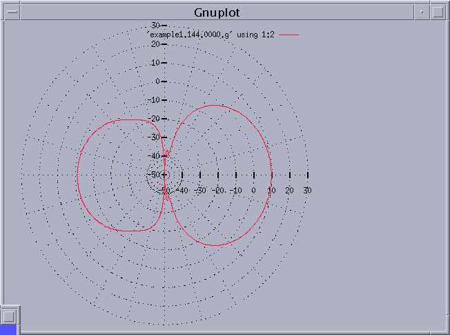
The -p option on output creates one file for every frequency step and files example1.glog and example1.glin that has commands for gnuplot (the well known grahpics package available from http://www.gnuplot.org/ ) The file 'example1.glog' shows the pattern on a logarathmic scale, as shown below.
parrot /export/home/drkirkby/yagiuda-1.18/src % gnuplot example1.gc
If an antenna has more than 20 dBi of gain, some of the graph will be missing. Similarily, an data below -50 dBi will not be shown. Use the -r and -R options on output to prevent this from happening. Hence to plot over -50 dBi to +30 dBi, use:
parrot /export/home/drkirkby/yagiuda-1.18/src % output -r -50
-R +30 -p example1
parrot /export/home/drkirkby/yagiuda-1.18/src % gnuplot example1.glog
File example1.glin shows the same data on a linear scale.
The antenna is not very good, so we will now optimise
it using optimise,
to improve its performance.